Create a workbook

1. Open Excel
2. Select Blank workbook or press Ctrl+N.
3. Start typing.

Create a workbook from a template

1. Select File > New.
2. Double-click a template.
3. Click and start typing.

Change Font, Style, Size, Colour, or Apply Effects

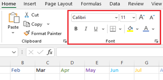
1. Click Home and:
2. For a different font style, click the arrow next to the default font Calibri and pick the style you want.
3. To increase or decrease the font size, click the arrow next to the default size 11 and pick another text size
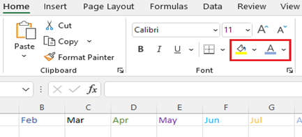
4. To change the font color, click Font Color and pick a color.
5. To add a background color, click Fill Color next to Font Color.
6. To apply strikethrough, superscript, or subscript formatting, click the Dialog Box Launcher, and select an option under Effects.

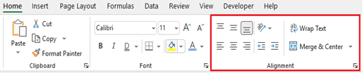
Change the text alignment

1. You can position the text within a cell so that it is centered, aligned left or right. If it’s a long line of text, you can apply Wrap Text so that all the text is visible.
2. Select the text that you want to align, and on the Home tab, pick the alignment option you want.

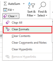
Clear formatting

1. If you change your mind after applying any formatting, to undo it, select the text, and on the Home tab, click Clear > Clear Formats.

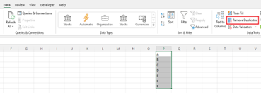
To remove duplicate values,

1. Click Data > Data Tools > Remove Duplicates.

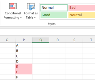
To highlight unique or duplicate values

1. Use the Conditional Formatting command in the Style group on the Home tab.


2. Select Highlight Cells Rules > Duplicate Values
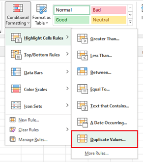
3. Any duplicates in the selected range will then be highlighted

The Transpose feature:

1. Select the range of data you want to rearrange, including any row or column labels, and either select Copy Copy icon on the Home tab, or press CONTROL+C.
2. Select the first cell where you want to paste the data, and on the Home tab, click the arrow next to Paste, and then click Transpose.
   • Pick a spot in the worksheet that has enough room to paste your data. The data you copied will overwrite any data that’s already there.
   
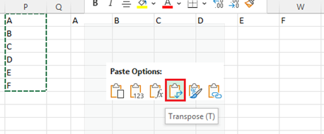
3. After rotating the data successfully, you can delete the original data.

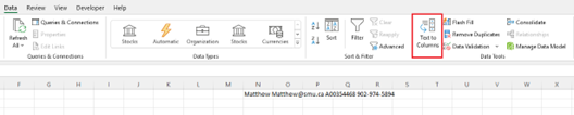
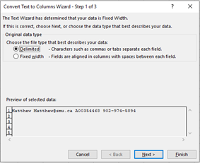
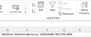
Delimiters:

1. Select the cell or column that contains the text you want to split.
2. Select Data and under Data Tools, select Text to Columns.
3. In the Convert Text to Columns Wizard, select Delimited > Next.
4. Select the Delimiters for your data. For example, Comma and Space. You can see a preview of your data in the Data preview
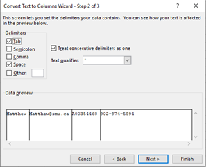
5. Select Next.
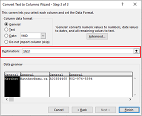
6. Select the Destination in your worksheet which is where you want the split data to appear.
7. Select Finish.

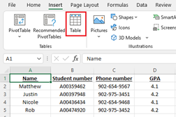
Turning your data into a table

1. Select the cells that contain the information for the table.
2. Click the Insert tab > Locate the "Tables" group.
3. Click Table.
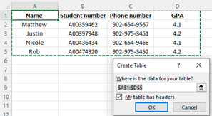
   • A "Create Table" dialog box will open.
4. If you have column headings, check the box My table has headers.
5. Verify that the range is correct > Click OK.
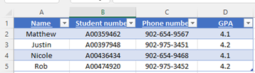
6. Resize your columns to make the headings visible.

AutoFill Sequences

1. Select one or more cells you want to use as a basis for filling additional cells.
   • For a series like 1, 2, 3, 4, 5..., type 1 and 2 in the first two cells. For the series 2, 4, 6, 8..., type 2 and 4.
   • For the series 2, 2, 2, 2..., type 2 in first cell only.
2. Drag the fill handle Fill handle.
3. If needed, click Auto Fill Options Button and choose the option you want.
4. And the series is filled in for you automatically using the AutoFill feature.

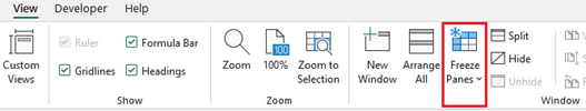
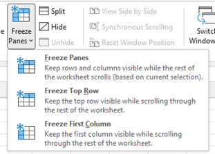
Freeze the first column

1. Select View > Freeze Panes > Freeze First Column.

Freeze the first two columns

1. Select the third column.
2. Select View > Freeze Panes > Freeze Panes.

Freeze columns and rows

1. Select the cell below the rows and to the right of the columns you want to keep visible when you scroll.
2. Select View > Freeze Panes > Freeze Panes.

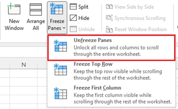
Unfreeze rows or columns

1. On the View tab > Window > Unfreeze Panes.

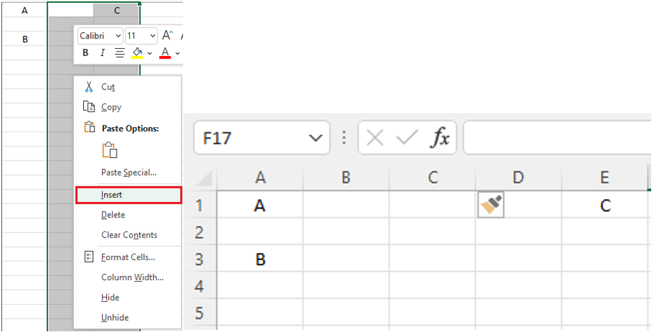
How to insert one or more rows/columns.

1. Select the row below where you want the new rows to appear.
2. Right click on the highlighted row and select "Insert" from the list. This will insert one row above the row you initially highlighted.
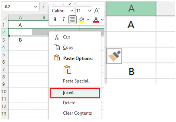
3. Add multiple rows or columns, highlight the same number of pre-existing rows or columns that you want to add. Then, right-click and select Insert.

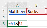
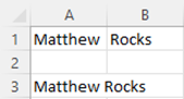
Combine Text from Multiple Cells

1. Select the cell in which you want the combined data
2. Type an = (equal sign) to start the formula
3. Click on the first cell
4. Type the & operator (shift + 7)
5. Click on the second cell
6. Press Enter to complete the formula

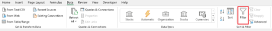
Adding a Filter

1. Select any cell within the range.
2. Select Data > Filter.
3. Select the column header arrow Filter arrow.
4. Select Text Filters or Number Filters, and then select a comparison, such as Between.
5. Enter the filter criteria and select OK.

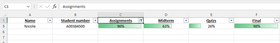
Filter data in a table

1. When you Create and format tables, filter controls are automatically added to the table headers.
2. Select the column header arrow Filter drop-down arrow for the column you want to filter.
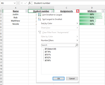
3. Uncheck (Select All) and select the boxes you want to show.
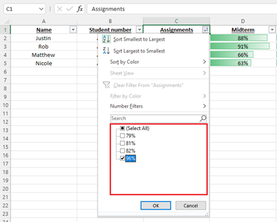
4. Click OK.
5. The column header arrow Filter drop-down arrow changes to a Applied filter icon Filter icon. Select this icon to change or clear the filter.

Conditional Formatting

1. Select the table or range where you want to change the background color of cells
2. Navigate to the Home tab, under Styles group, choose Conditional Formatting > New Rule….
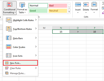
3. In the New Formatting Rule dialog box, select "Format only cells that contain" under "Select a Rule Type" box.
4. In the lower part of the dialog box under "Format Only Cells with section", set the rule conditions
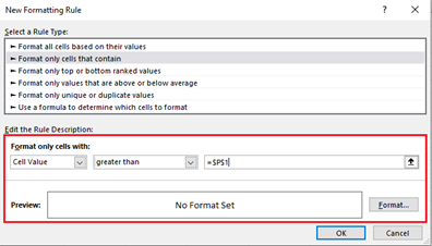
5. Click the Format
6. In the Format Cells dialog box, switch to the Fill tab and select the color of your choice
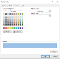
7. Click OK.
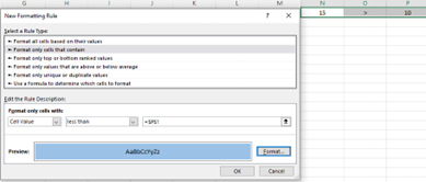
8. Back on the New Formatting Rule window, click OK

Equal sign:

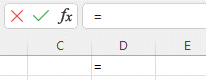
1. Before creating any formula, you’ll need to write an equal sign (=) in the cell where you want the result to appear.

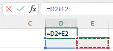
Addition:

1. To add the values of two or more cells, use the + sign. Example: =C1+D4.

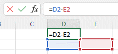
Subtraction:

1. To subtract the values of two or more cells, use the - sign. Example: =C1-D4.

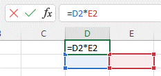
Multiplication:

1. To multiply the values of two or more cells, use the * sign. Example: =C1*D4.

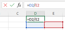
Division:

1. To divide the values of two or more cells, use the / sign. Example: =C1/D4.

Example: =(C1 - D4) / ((A5 + B6) * 3).

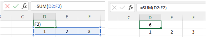
SUM:

1. The SUM function automatically adds up a range of cells or numbers. To complete a sum, you would input the starting cell and the final cell with a colon in between. Here’s what that looks like: SUM(Cell1:Cell2). Example: =SUM(C5:C30).

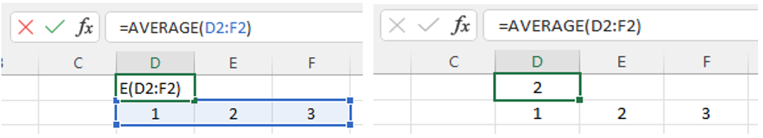
AVERAGE:

1. The AVERAGE function averages out the values of a range of cells. The syntax is the same as the SUM function: AVERAGE(Cell1:Cell2). Example: =AVERAGE(C5:C30).

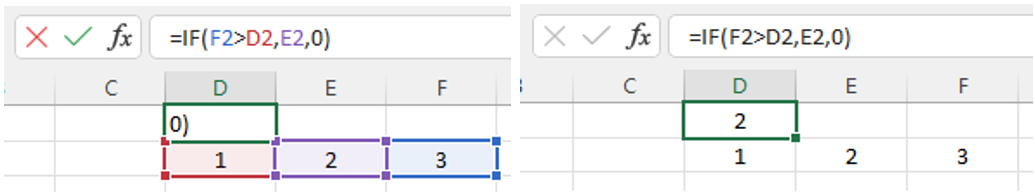
IF:

1. The IF function allows you to return values based on a logical test. The syntax is as follows: IF(logical_test, value_if_true, [value_if_false]). Example: =IF(A2>B2,"Over Budget","OK").

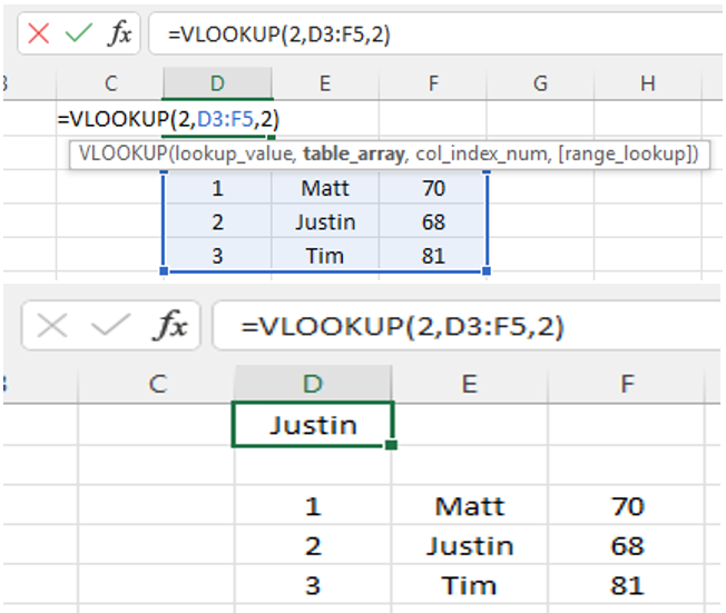
VLOOKUP:

1. The VLOOKUP function helps you search for anything on your sheet’s rows. The syntax is: VLOOKUP(lookup value, table array, column number, Approximate match (TRUE) or Exact match (FALSE)). Example: =VLOOKUP([@Attorney],tbl_Attorneys,4,FALSE).

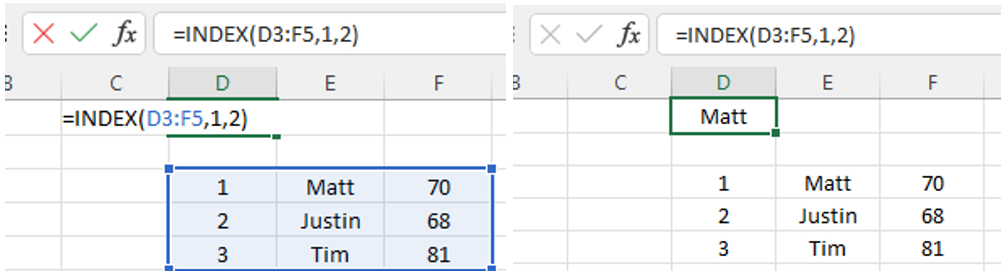
INDEX:

1. The INDEX function returns a value from within a range. The syntax is as follows: INDEX(array, row_num, [column_num]).

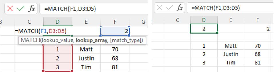
MATCH:

1. The MATCH function looks for a certain item in a range of cells and returns the position of that item. It can be used in tandem with the INDEX function. The syntax is: MATCH(lookup_value, lookup_array, match_type]).

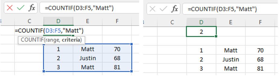
COUNTIF:

1. The COUNTIF function returns the number of cells that meet a certain criteria or have a certain value. The syntax is: COUNTIF(range, criteria). Example: =COUNTIF(A2:A5,"London").

Absolute Reference

1. The dollar sign ($) fixes the reference to a given cell, so that it remains unchanged no matter where the formula moves. In other words, using $ in cell references allows you to copy the formula in Excel without changing references.

Switch between absolute, relative, and mixed references (F4 key).

1. Select the cell you wish to edit.
2. Enter Edit mode by pressing the F2 key or double-click the cell.
3. Select the cell reference you want to change.
4. Press F4 to toggle between four cell reference types.

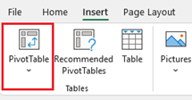
Create a PivotTable:

1. Select Insert > PivotTable.
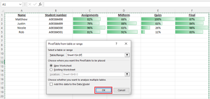
2. Under Select a table or range, In the Table/Range field, select the desired data for your chart.
3. Under Choose where you want the PivotTable report to be placed
   • Select New worksheet to place the PivotTable in a new worksheet or
   • Select Existing worksheet and then select the location you want the PivotTable to appear.
4. Select OK.

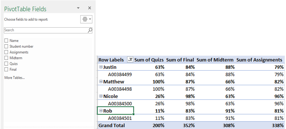
PivotTable Fields:

1. After you click OK on the PivotTable from the table or range you will be presented with options to add PivotTable Fields.
2. The Field List has a field section in which you pick the fields you want to show in your PivotTable.
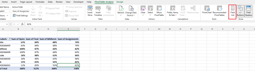
3. If you click inside the PivotTable but don't see the Field List, open it by clicking anywhere in the PivotTable. Then, select the PivotTable Analyze on the ribbon.
4. Click Field List.

PivotTable Options:

1. Report Filter: This allows you to only look at certain rows in your dataset.
2. Column Labels: These would be your headers in the dataset.
3. Row Labels: These could be your rows in the dataset. Both Row and Column labels can contain data from your
4. Value: This section allows you to look at your data differently. Instead of just pulling in any numeric value, you can sum, count, average, max, min, count numbers, or do a few other manipulations with your data. In fact, by default, when you drag a field to Value, it always does a count.

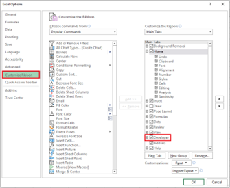
Developer Tag

1. Click File > Options > Customize Ribbon, select the Developer check box, and click OK.

Adding a Checkbox

1. To add a check box, click the Developer tab, click Insert, and under Form Controls, select the checkbox option.
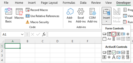
2. Click in the cell where you want to add the check box or option button control.
3. To edit or remove the default text for a control, click the control, and then update the text as needed.

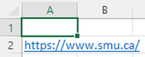
Inserting a Hyperlink

1. Press Shift K.
2. From there a box will pop up allowing you to place the hyperlink URL.
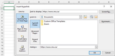
3. Copy and paste the URL into this box and hit OK or click Enter.

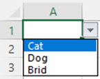
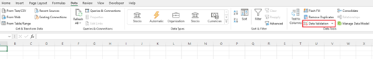
Data Validation

1. Highlight the cells you want the drop-downs to be in
2. Then click the Data menu in the top navigation
3. Under the Data Tools menu, click Data Validation.
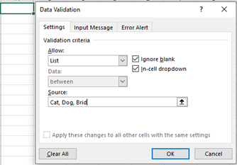
4. From there, you'll see a Data Validation Settings box
5. Under the Allow options, click Lists.
6. Check the In-Cell dropdown button.
7. Under Source you can enter data separated by a comma or select and highlight a field of cells that your drop-down menu will reference.
8. Press OK.